Chapter 5 Cell segmentation

Cell / nuclei segmentation is the task of identifying cells / nuclei in an appropriate image (we will be referring to cell and nuclei segmentation interchangeably here). There are numerous tools available for this purpose, but we will be covering two Python-based models specifically: cellpose (Stringer et al. 2021) and stardist (Schmidt et al. 2018; Weigert and Schmidt 2022).

As cell segmentation is performed on DAPI images, it can be performed in parallel with spotcalling.

library(masmr)
library(ggplot2)

## Warning: package 'ggplot2' was built under R version 4.3.2

5.1 Pre-processing

5.1.1 Establishing parameters

Similar to spotcalling, we first need to establish some parameters. The same code used for spotcalling can be repeated here.

data_dir = 'C:/Users/kwaje/Downloads/JIN_SIM/20190718_WK_T2_a_B2_R8_12_d50/'
establishParams(
  imageDirs = paste0(data_dir, 'S10/'),
  imageFormat = '.ome.tif',
  codebookFileName = list.files(paste0(data_dir, 'codebook/'), pattern='codebook', full.names = TRUE),
  codebookColumnNames = paste0(rep(c(0:3), 4), '_', rep(c('cy3', 'alexa594', 'cy5', 'cy7'), each=4) ),
  outDir = 'C:/Users/kwaje/Downloads/JYOUT/',
  dapiDir = paste0(data_dir, 'DAPI_1/'),
  pythonLocation = 'C:/Users/kwaje/AppData/Local/miniforge3/envs/scipyenv/',
  fpkmFileName = paste0(data_dir, "FPKM_data/Jin_FPKMData_B.tsv"),
  nProbesFileName = paste0(data_dir, "ProbesPerGene.csv"),
  verbose = FALSE
)

## Assuming .ome.tif is extension for meta files...

Of relevance to cell segmentation specifically are the pythonLocation and dapiDir parameters:

dapiDir: location of DAPI images. [Technically, any cell-based imaging will likely work here – not just DAPI – as long as they are compatible with the cell segmentation models.]
pythonLocation: location of the user’s Python environment. The Python environment should contain all the packages necessary to run the cell segmentation model of choice.

Details on the setting up of the Python environment is beyond the scope of this book. Briefly, there exist various tools (e.g. miniconda, anaconda, miniforge) that allow users to create a Python environment for installing necessary software. We will then interface with that environment through reticulate. Below are a series of commands to set up a Python environment called scipyenv that is compatible with stardist and cellpose. Users should take note of where the environment is created, and provide the location of the folder in pythonLocation.

conda create -n scipyenv python=3.9 notebook pandas numpy=1.26.4
conda activate scipyenv
conda install pytorch=1.12.1 cudatoolkit=10.2 -c pytorch #1.12.1 is the earliest mps is supported
pip install cellpose==3.0.11
pip install tensorflow==2.17.0
pip install stardist==0.9.1

Additionally, similar to spotcalling, we also readImageMetaData, though this time for DAPI images specifically. Because there will be no decoding, warnings about codebook column names not matching can be safely ignored.

readImageMetaData( 'dapi_dir' )

## Warning in readImageMetaData("dapi_dir"): Assuming this data has been acquired
## by Triton

## Warning in readImageMetaData("dapi_dir"): bit_name not matching
## codebookColumnNames: either edit GLOBALCOORD.csv or params$codebook_colnames
## (ignore this warning if codebook not needed, e.g. DAPI)

## Warning in readImageMetaData("dapi_dir"): Updating params$fov_names

## Warning in readImageMetaData("dapi_dir"): Unsuccessful attempt at correcting
## placeholder codebook column names (params$codebook_colnames)

As before, this adds additional metadata to the params object, albeit this time for DAPI images specifically:

print( params$resolutions )

## $per_pixel_microns
## [1] "0.0706" "0.0706"
## 
## $xydimensions_pixels
## [1] "2960" "2960"
## 
## $xydimensions_microns
## [1] "208.976" "208.976"
## 
## $channel_order
## [1] "dapi"
## 
## $fov_names
##   [1] "MMStack_1-Pos_000_000" "MMStack_1-Pos_001_000" "MMStack_1-Pos_002_000"
##   [4] "MMStack_1-Pos_003_000" "MMStack_1-Pos_004_000" "MMStack_1-Pos_005_000"
##   [7] "MMStack_1-Pos_006_000" "MMStack_1-Pos_007_000" "MMStack_1-Pos_008_000"
##  [10] "MMStack_1-Pos_009_000" "MMStack_1-Pos_009_001" "MMStack_1-Pos_008_001"
##  [13] "MMStack_1-Pos_007_001" "MMStack_1-Pos_006_001" "MMStack_1-Pos_005_001"
##  [16] "MMStack_1-Pos_004_001" "MMStack_1-Pos_003_001" "MMStack_1-Pos_002_001"
##  [19] "MMStack_1-Pos_001_001" "MMStack_1-Pos_000_001" "MMStack_1-Pos_000_002"
##  [22] "MMStack_1-Pos_001_002" "MMStack_1-Pos_002_002" "MMStack_1-Pos_003_002"
##  [25] "MMStack_1-Pos_004_002" "MMStack_1-Pos_005_002" "MMStack_1-Pos_006_002"
##  [28] "MMStack_1-Pos_007_002" "MMStack_1-Pos_008_002" "MMStack_1-Pos_009_002"
##  [31] "MMStack_1-Pos_009_003" "MMStack_1-Pos_008_003" "MMStack_1-Pos_007_003"
##  [34] "MMStack_1-Pos_006_003" "MMStack_1-Pos_005_003" "MMStack_1-Pos_004_003"
##  [37] "MMStack_1-Pos_003_003" "MMStack_1-Pos_002_003" "MMStack_1-Pos_001_003"
##  [40] "MMStack_1-Pos_000_003" "MMStack_1-Pos_000_004" "MMStack_1-Pos_001_004"
##  [43] "MMStack_1-Pos_002_004" "MMStack_1-Pos_003_004" "MMStack_1-Pos_004_004"
##  [46] "MMStack_1-Pos_005_004" "MMStack_1-Pos_006_004" "MMStack_1-Pos_007_004"
##  [49] "MMStack_1-Pos_008_004" "MMStack_1-Pos_009_004" "MMStack_1-Pos_009_005"
##  [52] "MMStack_1-Pos_008_005" "MMStack_1-Pos_007_005" "MMStack_1-Pos_006_005"
##  [55] "MMStack_1-Pos_005_005" "MMStack_1-Pos_004_005" "MMStack_1-Pos_003_005"
##  [58] "MMStack_1-Pos_002_005" "MMStack_1-Pos_001_005" "MMStack_1-Pos_000_005"
##  [61] "MMStack_1-Pos_000_006" "MMStack_1-Pos_001_006" "MMStack_1-Pos_002_006"
##  [64] "MMStack_1-Pos_003_006" "MMStack_1-Pos_004_006" "MMStack_1-Pos_005_006"
##  [67] "MMStack_1-Pos_006_006" "MMStack_1-Pos_007_006" "MMStack_1-Pos_008_006"
##  [70] "MMStack_1-Pos_009_006" "MMStack_1-Pos_009_007" "MMStack_1-Pos_008_007"
##  [73] "MMStack_1-Pos_007_007" "MMStack_1-Pos_006_007" "MMStack_1-Pos_005_007"
##  [76] "MMStack_1-Pos_004_007" "MMStack_1-Pos_003_007" "MMStack_1-Pos_002_007"
##  [79] "MMStack_1-Pos_001_007" "MMStack_1-Pos_000_007" "MMStack_1-Pos_000_008"
##  [82] "MMStack_1-Pos_001_008" "MMStack_1-Pos_002_008" "MMStack_1-Pos_003_008"
##  [85] "MMStack_1-Pos_004_008" "MMStack_1-Pos_005_008" "MMStack_1-Pos_006_008"
##  [88] "MMStack_1-Pos_007_008" "MMStack_1-Pos_008_008" "MMStack_1-Pos_009_008"
##  [91] "MMStack_1-Pos_009_009" "MMStack_1-Pos_008_009" "MMStack_1-Pos_007_009"
##  [94] "MMStack_1-Pos_006_009" "MMStack_1-Pos_005_009" "MMStack_1-Pos_004_009"
##  [97] "MMStack_1-Pos_003_009" "MMStack_1-Pos_002_009" "MMStack_1-Pos_001_009"
## [100] "MMStack_1-Pos_000_009"
## 
## $zslices
## [1] "1"

knitr::kable( head( params$global_coords ), format = 'html', booktabs = TRUE )

x_microns	y_microns	z_microns	image_file	fov	bit_name_full	bit_name_alias	bit_name
-2645.753	3421.847	5678.52	C:/Users/kwaje/Downloads/JIN_SIM/20190718_WK_T2_a_B2_R8_12_d50/DAPI_1/DAPI_1_MMStack_1-Pos_000_000.ome.tif	MMStack_1-Pos_000_000	DAPI_1_dapi	0_dapi	DAPI_1_dapi
-2645.753	3609.926	5678.54	C:/Users/kwaje/Downloads/JIN_SIM/20190718_WK_T2_a_B2_R8_12_d50/DAPI_1/DAPI_1_MMStack_1-Pos_000_001.ome.tif	MMStack_1-Pos_000_001	DAPI_1_dapi	0_dapi	DAPI_1_dapi
-2645.753	3798.004	5678.56	C:/Users/kwaje/Downloads/JIN_SIM/20190718_WK_T2_a_B2_R8_12_d50/DAPI_1/DAPI_1_MMStack_1-Pos_000_002.ome.tif	MMStack_1-Pos_000_002	DAPI_1_dapi	0_dapi	DAPI_1_dapi
-2645.753	3986.082	5678.58	C:/Users/kwaje/Downloads/JIN_SIM/20190718_WK_T2_a_B2_R8_12_d50/DAPI_1/DAPI_1_MMStack_1-Pos_000_003.ome.tif	MMStack_1-Pos_000_003	DAPI_1_dapi	0_dapi	DAPI_1_dapi
-2645.753	4174.161	5678.60	C:/Users/kwaje/Downloads/JIN_SIM/20190718_WK_T2_a_B2_R8_12_d50/DAPI_1/DAPI_1_MMStack_1-Pos_000_004.ome.tif	MMStack_1-Pos_000_004	DAPI_1_dapi	0_dapi	DAPI_1_dapi
-2645.753	4362.239	5678.38	C:/Users/kwaje/Downloads/JIN_SIM/20190718_WK_T2_a_B2_R8_12_d50/DAPI_1/DAPI_1_MMStack_1-Pos_000_005.ome.tif	MMStack_1-Pos_000_005	DAPI_1_dapi	0_dapi	DAPI_1_dapi

5.1.2 Establishing the cell segmentation model

Unique to the cell segmentation script, users must load their desired cell segmentation model into the environment. This is accomplished with the establishCellSegModel function, which returns a new environment object called cellSeg.

If no other parameters are specified, the nuclei model in cellpose is loaded. [We will showcase loading different models later in this chapter.] Additionally, GPU acceleration is turned off as default – users able to access their computer’s GPU may turn this on for time saving.

establishCellSegModel()

## 
## Preparing cell segmentation model(s)...

## Cellpose packaged model...

The cellSeg environment keeps track of which model has been loaded and the outputs expected from that model. Users may load multiple models if they so wish but this will increase the run time: all models in cellSeg will be run on DAPI images. Below, we have a single model CELLPOSE, within which we have the model and the expected outputs.

ls(cellSeg)

## [1] "CELLPOSE"

cellSeg$CELLPOSE

## $model
## <cellpose.models.CellposeModel object at 0x000001DA04F987C0>
## 
## $outputs
## [1] "masks"  "flows"  "styles" "diams"

5.2 Running cell segmentation

For memory management, it is recommended that FOVs are processed as individual tiles. Below, we read in a specific FOV (and as recommended, save the current FOV in params$current_fov). We can use readImage for a specific file, or – if we know which FOV we want – with readImageList.

NOTE: below may be more complicated for Z-stacks and multiple channels. Process accordingly so thatimis a single matrix of the DAPI channel.

params$current_fov <- params$fov_names[38]
im <- readImageList( params$current_fov )[[1]] #List of 1
plot(imager::as.cimg(im))

## Warning in as.cimg.array(im): Assuming third dimension corresponds to
## time/depth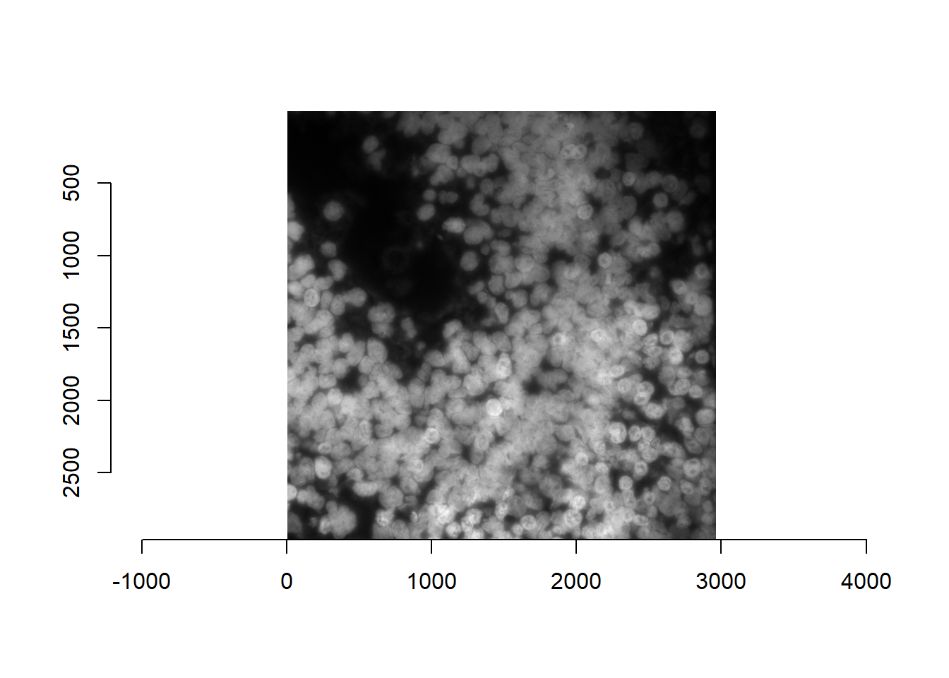

5.3 Running segmentation model

Once the necessary parameters have been established, we are ready to run our cell segmentation model with the runCellSegModel function. Further image processing of DAPI images generally is not necessary as these models tend to have in-built image processing functions. However, we have found that modifying image parameters can influence cell segmentation; a more detailed discussion is provided below.

5.3.1 `cellpose`

cellpose is our default choice owing to it being applicable to both nuclei and cellular segmentation. It is a deep-learning based segmentation model trained on a variety of image types including DAPI images alone (nuclei), and multi-channel images with both nuclei and cell boundary stains (cyto, cyto2, and cyto3).

An example of how to run the model within masmr is shown below. [As default, only the mask output is returned; this can be turned off by setting masksOnly to FALSE.]

cellMask <- runCellSegModel(im, masksOnly = TRUE)
df <- as.data.frame(imager::as.cimg(cellMask))
ggplot() +
  geom_raster( data = as.data.frame(imager::as.cimg(im)), 
               aes(x=x, y=y, fill=value) ) +
  scale_fill_gradient(low='black', high='white') +
  geom_point( data=df[df$value>0,], 
              aes(x=x, y=y, colour=factor(value)),
              shape = '.') +
  scale_colour_viridis_d( option='turbo' ) +
  theme_void( base_size = 14 ) +
  scale_y_reverse() +
  coord_fixed() +
  theme(legend.position = 'none')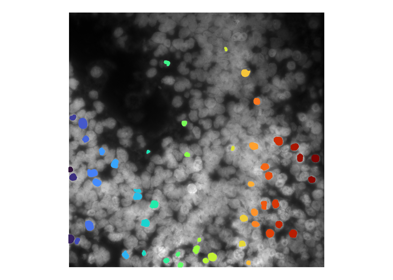

The default nuclei model called for cellpose does not seem to be working very well for these images. There are several ways to troubleshoot:

Dilating existing masks

If the issue is that cell masks are accurate, but too small – which would lower the number of counts assigned to each cell – one quick solution would be to dilate the existing masks.

There are several ways to do this. Below is an example of how to do this quickly with imager – which is a dependency of masmr. [Possible alternatives: Voronoi tessellation, setting a radius threshold from the cell segmentation mask centre.]

dilation_sizes <- c(0L, 50L)
plotList <- list()
for(i in 1:length(dilation_sizes)){
  
  ## Dilate a cellMask by a certain size
  original_cellMask <- imager::as.cimg(cellMask)
  dilated_cellMask <- imager::dilate_square(original_cellMask, size = dilation_sizes[i] )
  
  ## Plot the masks atop the original image
  df <- as.data.frame(dilated_cellMask)
  plotList[[i]] <- ggplot() +
    geom_raster( data = as.data.frame(imager::as.cimg(im)), 
                 aes(x=x, y=y, fill=value) ) +
    scale_fill_gradient(low='black', high='white') +
    geom_point( data=df[df$value>0,], 
                aes(x=x, y=y, colour=factor(value)),
                shape = '.') +
    scale_colour_viridis_d( option='turbo' ) +
    theme_void( base_size = 14 ) +
    scale_y_reverse() +
    coord_fixed() +
    theme(legend.position = 'none') +
    ggtitle( paste0('Dilate size: ', dilation_sizes[i] ))
}
cowplot::plot_grid(plotlist = plotList)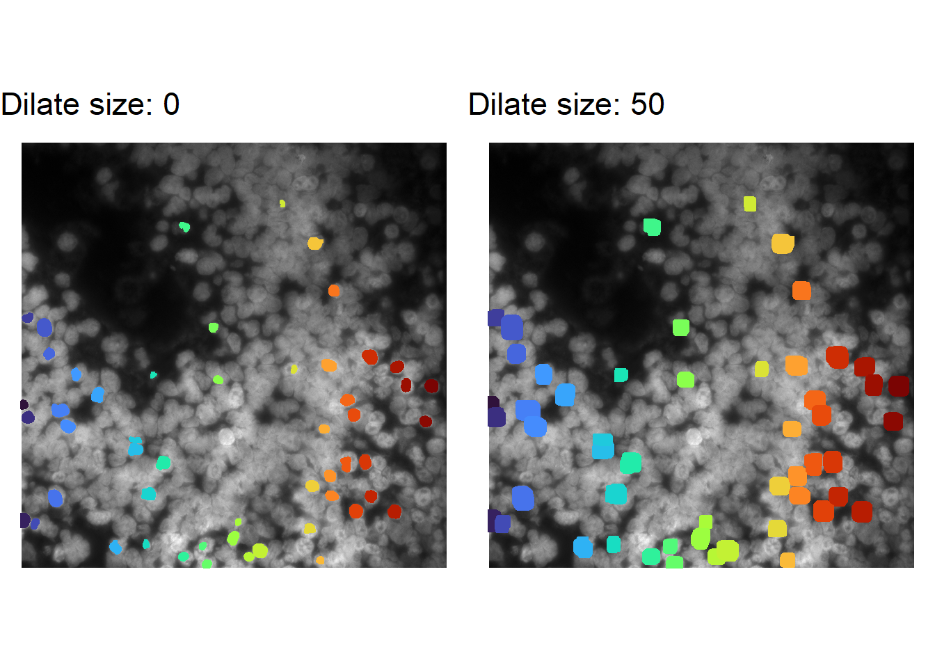

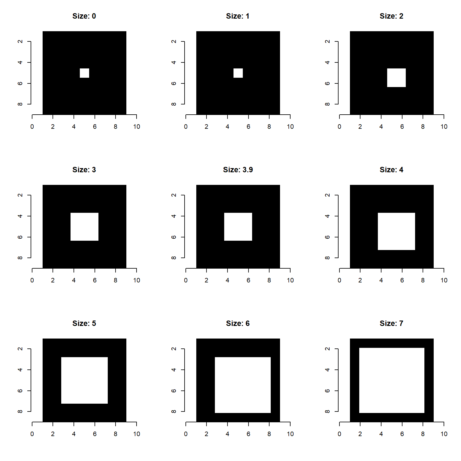
Note: the choice of the size parameter for imager::dilate_square is slightly non-intuitive: (1) input values are rounded down to the nearest integer, and (2) odd numbers provide isotropic dilations (even values dilate to the bottom right).

pretendImage <- imager::as.cimg( array(0, dim=c(9, 9)) )
pretendImage[5,5] <- 1
dilation_sizes <- c(0, 1, 2, 3, 3.9, 4, 5, 6, 7)
par(mfrow=c(3,3))
for( i in 1:length(dilation_sizes) ){
  plot( imager::dilate_square(pretendImage, size=dilation_sizes[i]), interpolate=F,
        main = paste0('Size: ', dilation_sizes[i]) )
}

par(mfrow=c(1,1))

Altering model parameters

The default evaluation for cellpose assumes a diameter of 30 pixels. If we wish to increase this value, this can be accomplished by adding model parameters to runCellSegModel. Below, we increase the diameter parameter (specific to the cellpose model) to 50. [masksOnly is default TRUE, will not reproduce that parameter below.]

cellMask <- runCellSegModel(im, diameter = 50)
df <- as.data.frame(imager::as.cimg(cellMask))
ggplot() +
  geom_raster( data = as.data.frame(imager::as.cimg(im)), 
               aes(x=x, y=y, fill=value) ) +
  scale_fill_gradient(low='black', high='white') +
  geom_point( data=df[df$value>0,], 
              aes(x=x, y=y, colour=factor(value)),
              shape = '.') +
  scale_colour_viridis_d( option='turbo' ) +
  theme_void( base_size = 14 ) +
  scale_y_reverse() +
  coord_fixed() +
  theme(legend.position = 'none')

## Warning in as.cimg.array(im): Assuming third dimension corresponds to
## time/depth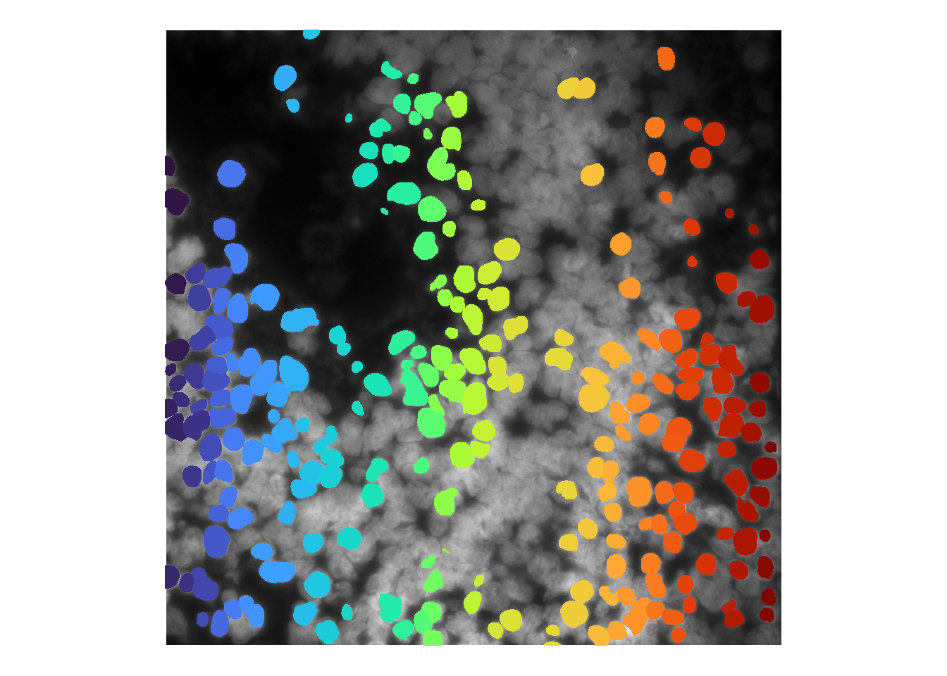

Image processing

For some models, altering the intensity values (e.g. by brightening) can influence model performance. For cellpose, the model is generally robust to additional image processing. [Compare to stardist below.]

norm <- im^0.5
par(mfrow=c(1,2))
plot(imager::as.cimg(im), main = 'Original image')

## Warning in as.cimg.array(im): Assuming third dimension corresponds to
## time/depth

plot(imager::as.cimg(norm), main = 'Brightened image')

## Warning in as.cimg.array(norm): Assuming third dimension corresponds to
## time/depth

par(mfrow=c(1,1))

cellMask <- runCellSegModel( norm )
df <- as.data.frame(imager::as.cimg(cellMask))
ggplot() +
  geom_raster( data = as.data.frame(imager::as.cimg(im)), 
               aes(x=x, y=y, fill=value) ) +
  scale_fill_gradient(low='black', high='white') +
  geom_point( data=df[df$value>0,], 
              aes(x=x, y=y, colour=factor(value)),
              shape = '.') +
  scale_colour_viridis_d( option='turbo' ) +
  theme_void( base_size = 14 ) +
  scale_y_reverse() +
  coord_fixed() +
  theme(legend.position = 'none')

## Warning in as.cimg.array(im): Assuming third dimension corresponds to
## time/depth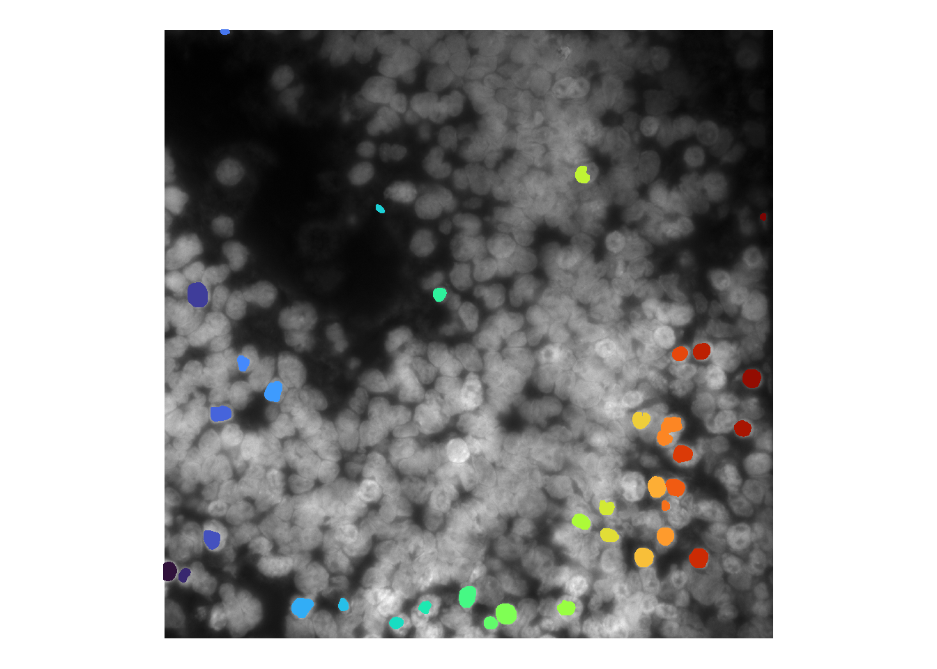

Loading a retrained model

If users have the resources to retrain the default cellpose model (Pachitariu and Stringer 2022), this retrained model can be loaded in lieu of the default models. To do so, user’s model can be specified in establishCellSegModel.

[Model retraining is beyond the scope of this book. Users are encouraged to look up the documentation for cellpose.]

establishCellSegModel(
  cellposePreTrainedModel =
    'C:/Users/kwaje/OneDrive - A STAR/Documents/Workplace/Liu_Connect/Code/jinyue_cellpose_models/CP_model3_newB4_800epoch_lr0pt01_FINAL'
)

## 
## Preparing cell segmentation model(s)...

## User-pretrained Cellpose model...

cellMask <- runCellSegModel(im)
df <- as.data.frame(imager::as.cimg(cellMask))
ggplot() +
  geom_raster( data = as.data.frame(imager::as.cimg(im)), 
               aes(x=x, y=y, fill=value) ) +
  scale_fill_gradient(low='black', high='white') +
  geom_point( data=df[df$value>0,], 
              aes(x=x, y=y, colour=factor(value)),
              shape = '.') +
  scale_colour_viridis_d( option='turbo' ) +
  theme_void( base_size = 14 ) +
  scale_y_reverse() +
  coord_fixed() +
  theme(legend.position = 'none')

## Warning in as.cimg.array(im): Assuming third dimension corresponds to
## time/depth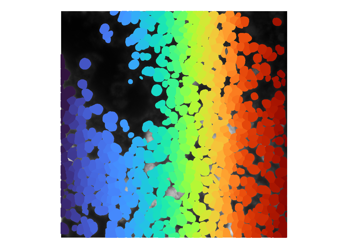

5.3.2 `stardist`

An alternative for nuclei segmentation is to use stardist: a deep-learning segmentation model that relies on star-convex polygons. The model has been trained on DAPI images (2D_versatile_fluo), and H&E stains (2D_versatile_he). It is typically faster than cellpose, allowing for looping through multiple hyperparameters – should users be interested.

[Tip: Windows users have reported running into [WinError 1314] A required privilege is not held by the client error when attempting to load stardist. To get around the problem, manually unzip the downloaded model (file location reported in error message). For some reason, 2D_versatile_fluo.zip is erroneously unzipped as 2D_versatile_fluo_extracted instead of 2D_versatile_fluo in some cases.]

establishCellSegModel( 'stardist' )

## 
## Preparing cell segmentation model(s)...

## Stardist packaged model...

## Found model '2D_versatile_fluo' for 'StarDist2D'.
## Loading network weights from 'weights_best.h5'.
## Loading thresholds from 'thresholds.json'.
## Using default values: prob_thresh=0.479071, nms_thresh=0.3.

cellMask <- runCellSegModel(im)
df <- as.data.frame(imager::as.cimg(cellMask))
ggplot() +
  geom_raster( data = as.data.frame(imager::as.cimg(im)), 
               aes(x=x, y=y, fill=value) ) +
  scale_fill_gradient(low='black', high='white') +
  geom_point( data=df[df$value>0,], 
              aes(x=x, y=y, colour=factor(value)),
              shape = '.') +
  scale_colour_viridis_d( option='turbo' ) +
  theme_void( base_size = 14 ) +
  scale_y_reverse() +
  coord_fixed() +
  theme(legend.position = 'none')

## Warning in as.cimg.array(im): Assuming third dimension corresponds to
## time/depth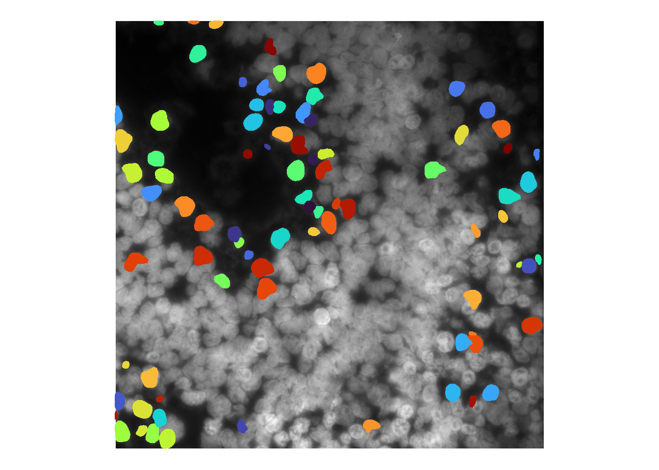

As with cellpose, there are various ways to troubleshoot base stardist performance.

Like cellpose, users can tweak stardist model parameters during runCellSegModel. For instance, decreasing prob_thresh (default: 0.48) increases sensitivity.

cellMask <- runCellSegModel(im, prob_thresh = 0.1)
df <- as.data.frame(imager::as.cimg(cellMask))
ggplot() +
  geom_raster( data = as.data.frame(imager::as.cimg(im)), 
               aes(x=x, y=y, fill=value) ) +
  scale_fill_gradient(low='black', high='white') +
  geom_point( data=df[df$value>0,], 
              aes(x=x, y=y, colour=factor(value)),
              shape = '.') +
  scale_colour_viridis_d( option='turbo' ) +
  theme_void( base_size = 14 ) +
  scale_y_reverse() +
  coord_fixed() +
  theme(legend.position = 'none')

## Warning in as.cimg.array(im): Assuming third dimension corresponds to
## time/depth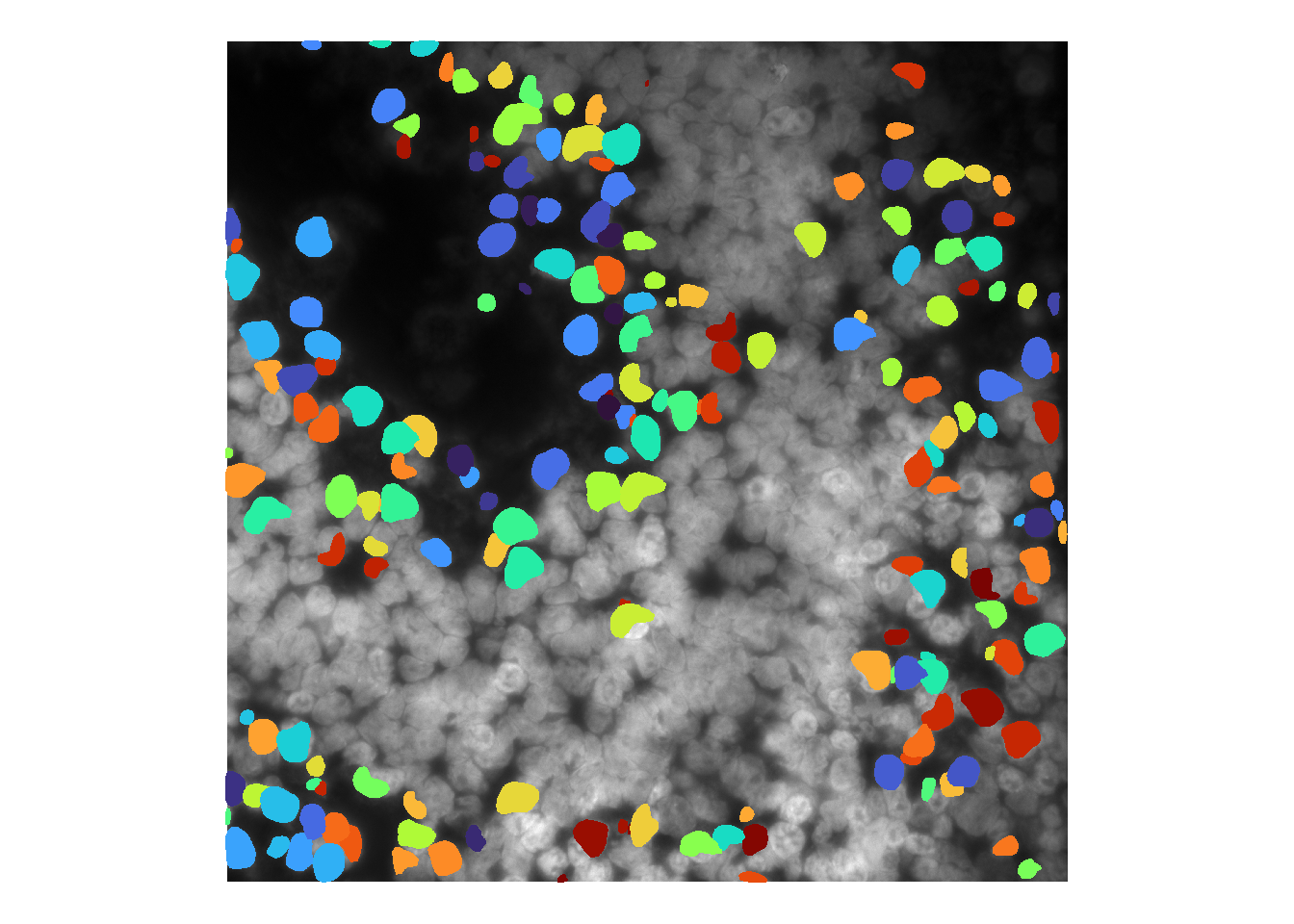

We have also found stardist to be more sensitive to brightness values / image processing than cellpose. For instance, brightening the image as before greatly impairs nuclei detection:

norm <- im^0.5
par(mfrow=c(1,2))
plot(imager::as.cimg(im), main = 'Original image')

## Warning in as.cimg.array(im): Assuming third dimension corresponds to
## time/depth

plot(imager::as.cimg(norm), main = 'Brightened image')

## Warning in as.cimg.array(norm): Assuming third dimension corresponds to
## time/depth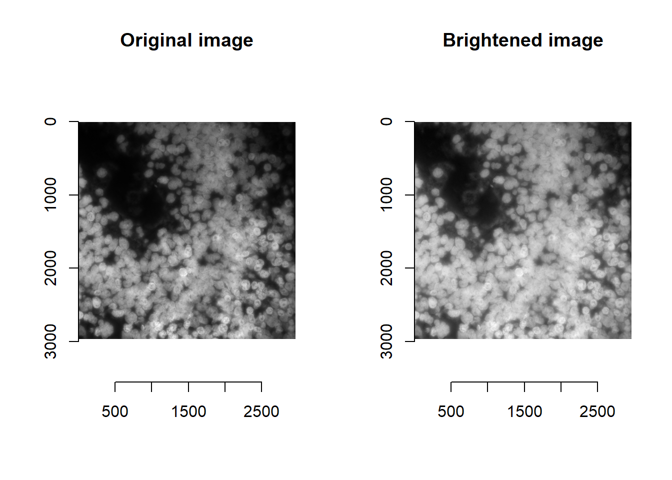

par(mfrow=c(1,1))

cellMask <- runCellSegModel( norm )
df <- as.data.frame(imager::as.cimg(cellMask))
ggplot() +
  geom_raster( data = as.data.frame(imager::as.cimg(im)), 
               aes(x=x, y=y, fill=value) ) +
  scale_fill_gradient(low='black', high='white') +
  geom_point( data=df[df$value>0,], 
              aes(x=x, y=y, colour=factor(value)),
              shape = '.') +
  scale_colour_viridis_d( option='turbo' ) +
  theme_void( base_size = 14 ) +
  scale_y_reverse() +
  coord_fixed() +
  theme(legend.position = 'none')

## Warning in as.cimg.array(im): Assuming third dimension corresponds to
## time/depth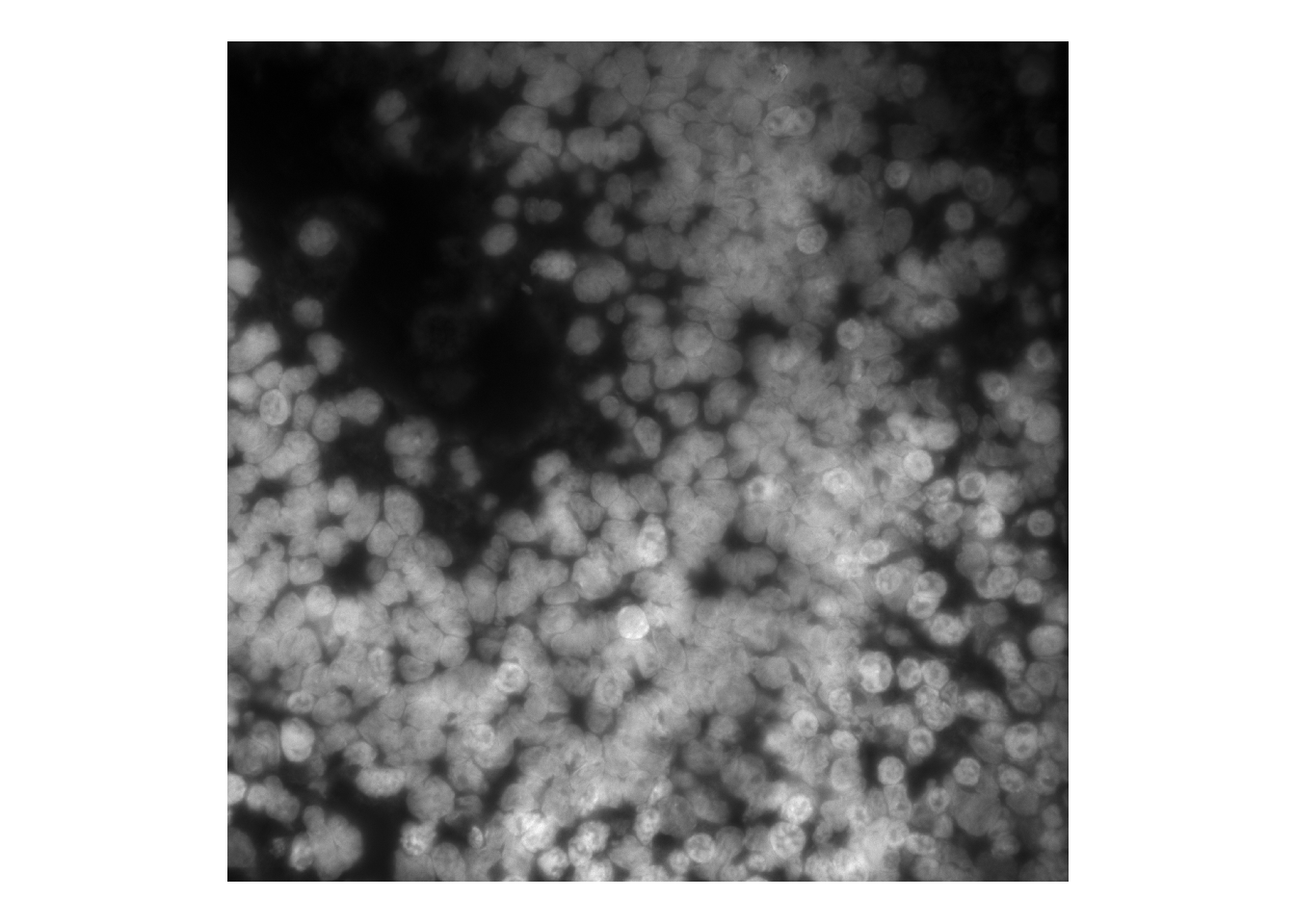

And darkening the image greatly increases sensitivity:

norm <- im^1.5
par(mfrow=c(1,2))
plot(imager::as.cimg(im), main = 'Original image')

## Warning in as.cimg.array(im): Assuming third dimension corresponds to
## time/depth

plot(imager::as.cimg(norm), main = 'Darkened image')

## Warning in as.cimg.array(norm): Assuming third dimension corresponds to
## time/depth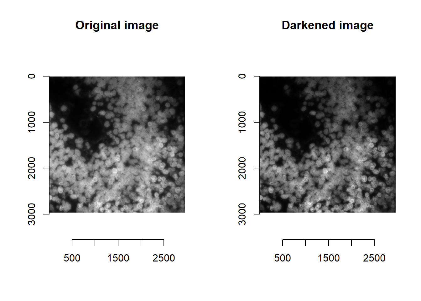

par(mfrow=c(1,1))

cellMask <- runCellSegModel( norm )
df <- as.data.frame(imager::as.cimg(cellMask))
ggplot() +
  geom_raster( data = as.data.frame(imager::as.cimg(im)), 
               aes(x=x, y=y, fill=value) ) +
  scale_fill_gradient(low='black', high='white') +
  geom_point( data=df[df$value>0,], 
              aes(x=x, y=y, colour=factor(value)),
              shape = '.') +
  scale_colour_viridis_d( option='turbo' ) +
  theme_void( base_size = 14 ) +
  scale_y_reverse() +
  coord_fixed() +
  theme(legend.position = 'none')

## Warning in as.cimg.array(im): Assuming third dimension corresponds to
## time/depth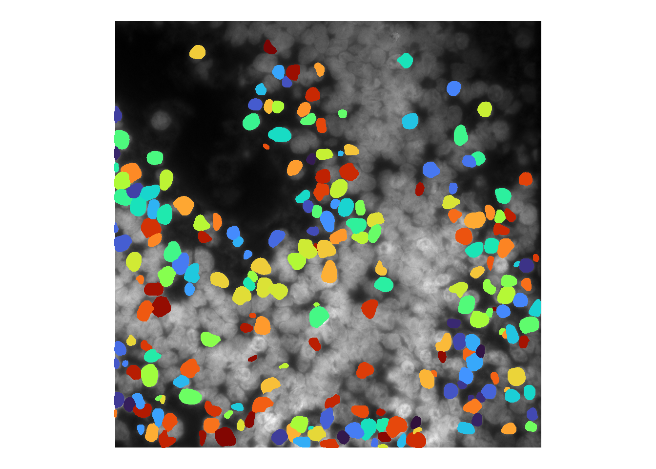

Given this sensitivity, and the relatively faster speed of stardist, users might wish to try different image processing prior to cell segmentation. This can be accomplished as below. Note that runCellSegModel accepts both a single image matrix, and a list of images. [The same is achievable for cellpose if desired, but users should be aware of the longer runtime.]

powerValues <- seq(0.5, 2, length.out = 6)
par(mfrow=c(2, 3))
imList <- lapply( powerValues, function(x){ 
  norm <- im^x
  plot( imager::as.cimg(norm), main = paste0('Image ^ ', round(x, digits=1) ) ) 
  return(norm)
  })

## Warning in as.cimg.array(norm): Assuming third dimension corresponds to
## time/depth

## Warning in as.cimg.array(norm): Assuming third dimension corresponds to
## time/depth

## Warning in as.cimg.array(norm): Assuming third dimension corresponds to
## time/depth

## Warning in as.cimg.array(norm): Assuming third dimension corresponds to
## time/depth

## Warning in as.cimg.array(norm): Assuming third dimension corresponds to
## time/depth

## Warning in as.cimg.array(norm): Assuming third dimension corresponds to
## time/depth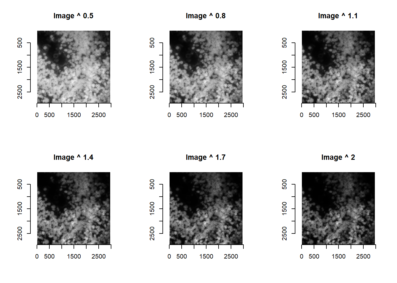

names( imList ) <- paste0("Power", round(powerValues, digits=1))

cellMasks <- runCellSegModel( imList )
for(i in 1:length(cellMasks)){
  plot( imager::as.cimg(cellMasks[[i]]), main = paste0('Masks of ', names(cellMasks)[i]) )
}

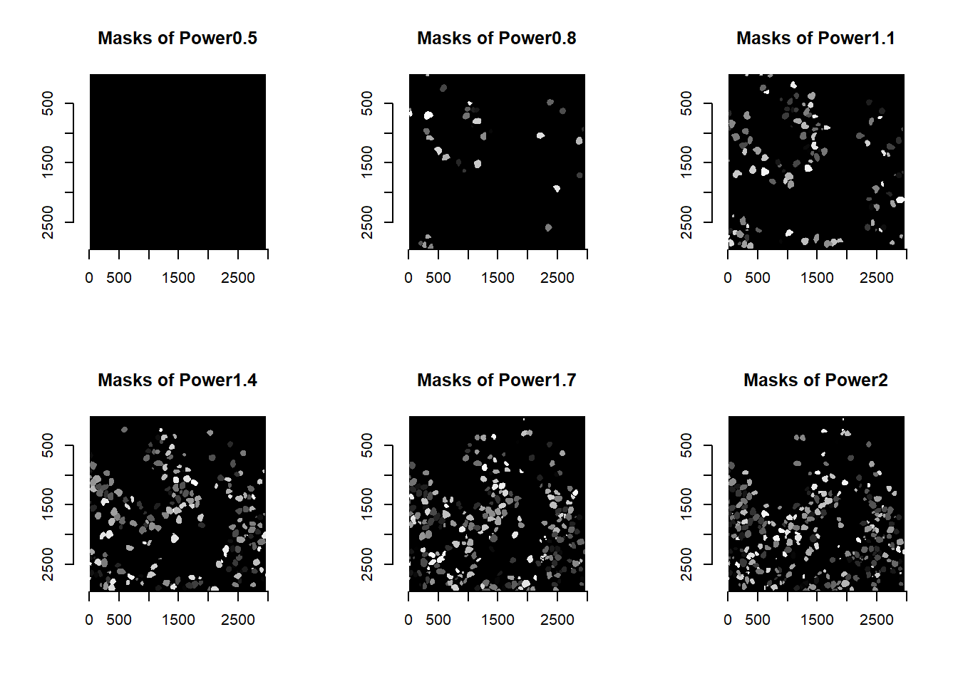
par(mfrow=c(1, 1))

To summarise a list of masks into a single mask matrix, we provide the consolidateCellSegMasks function. This works by overlaying all masks in the list, and only accepting image pixels that have been masked at least $n$ times. As default, $n = 1$, so if a pixel is masked at least once, it is brought forwards.

cellMask <- consolidateCellSegMasks( cellMasks )
df <- as.data.frame(imager::as.cimg(cellMask))
ggplot() +
  geom_raster( data = as.data.frame(imager::as.cimg(im)), 
               aes(x=x, y=y, fill=value) ) +
  scale_fill_gradient(low='black', high='white') +
  geom_point( data=df[df$value>0,], 
              aes(x=x, y=y, colour=factor(value)),
              shape = '.') +
  scale_colour_viridis_d( option='turbo' ) +
  theme_void( base_size = 14 ) +
  scale_y_reverse() +
  coord_fixed() +
  theme(legend.position = 'none')

## Warning in as.cimg.array(im): Assuming third dimension corresponds to
## time/depth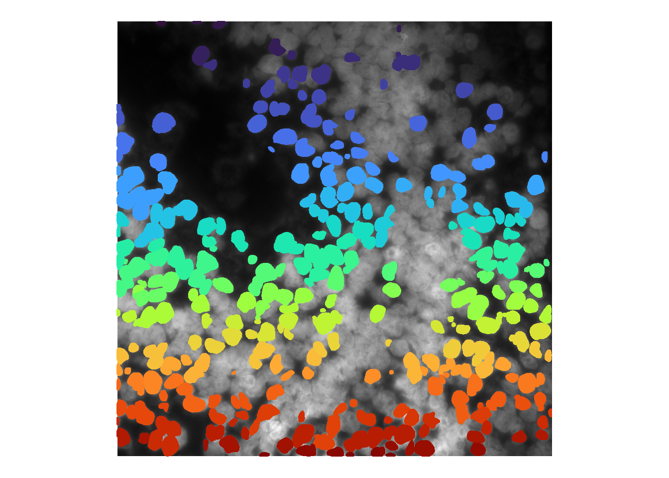

Increasing $n$ means pixels need to be masked more than once, and thus decreases the number of masks identified. Below shows $n = 2$:

cellMask <- consolidateCellSegMasks( cellMasks, minFlags = 2 )
df <- as.data.frame(imager::as.cimg(cellMask))
ggplot() +
  geom_raster( data = as.data.frame(imager::as.cimg(im)), 
               aes(x=x, y=y, fill=value) ) +
  scale_fill_gradient(low='black', high='white') +
  geom_point( data=df[df$value>0,], 
              aes(x=x, y=y, colour=factor(value)),
              shape = '.') +
  scale_colour_viridis_d( option='turbo' ) +
  theme_void( base_size = 14 ) +
  scale_y_reverse() +
  coord_fixed() +
  theme(legend.position = 'none')

## Warning in as.cimg.array(im): Assuming third dimension corresponds to
## time/depth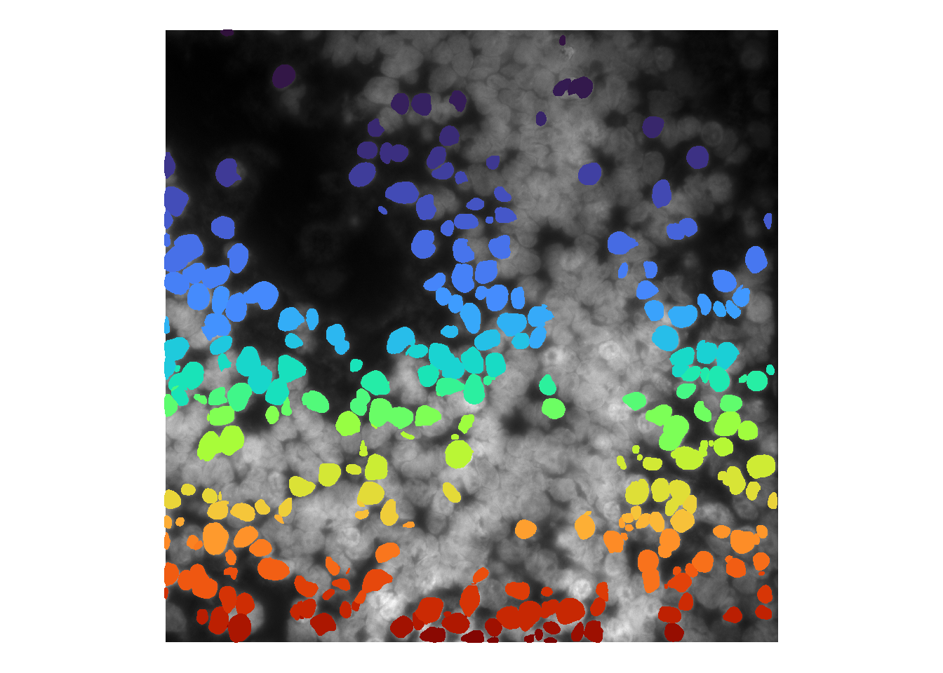

5.4 Saving cell masks

If users are satisfied with model performance, they can use saveCellSegMasks to save masks as a .csv.gz file. Additionally, it is recommended that users save the DAPI image used for cell segmentation. As default, the last image to be processed is stored under params$cell_seg_image, and will be saved if no other images are specified for saveCellSegMasks.

par(mfrow=c(1,2))
plot( imager::as.cimg(im), main = 'Original image' )

## Warning in as.cimg.array(im): Assuming third dimension corresponds to
## time/depth

plot( imager::as.cimg(params$cell_seg_image), main = 'Last image processed' )

## Warning in as.cimg.array(params$cell_seg_image): Assuming third dimension
## corresponds to time/depth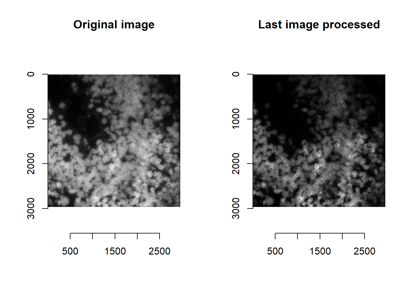

par(mfrow=c(1,1))

Saving cell masks creates a CELLSEG_{ Cell segmentation model }_{ FOV name }.csv.gz file containing masks, and a REGIM_{ FOV Name }.png image (depending on what is input into the im parameter).

saveCellSegMasks(cellMask, im = im)
file.exists( paste0(params$out_dir, 'REGIM_', params$current_fov, '.png') )

## [1] TRUE

References

Pachitariu, Marius, and Carsen Stringer. 2022. “Cellpose 2.0: How to Train Your Own Model.” Nature Methods 19 (12): 1634–41.

Schmidt, Uwe, Martin Weigert, Coleman Broaddus, and Gene Myers. 2018. “Cell Detection with Star-Convex Polygons.” In Medical Image Computing and Computer Assisted Intervention–MICCAI 2018: 21st International Conference, Granada, Spain, September 16-20, 2018, Proceedings, Part II 11, 265–73. Springer.

Stringer, Carsen, Tim Wang, Michalis Michaelos, and Marius Pachitariu. 2021. “Cellpose: A Generalist Algorithm for Cellular Segmentation.” Nature Methods 18 (1): 100–106.

Weigert, Martin, and Uwe Schmidt. 2022. “Nuclei Instance Segmentation and Classification in Histopathology Images with Stardist.” In 2022 IEEE International Symposium on Biomedical Imaging Challenges (ISBIC), 1–4. IEEE.